Fisher Information Part 1 - Some Intuition
Fisher Information is one of those topics that many will cover once in their studies on the way to more applied areas of statistics. The practical use of the CRLB is limited to cases where the sample at hand has a known distribution with an analytic form, which often doesn’t apply.
These posts will take a brief look at the Fisher Information and the CRLB from a less formal point of view to gain some intuitive sense of what they are doing.
Score
The score can be calculated as:
$$ V\left( X,\theta \right) =\dfrac{\partial }{\partial \theta }\ln L\left( X,\theta \right) $$
A good way of thinking about score is as sensitivity of the log-likelihood to $\theta$ at a specific value of $\theta$. In other words, a large score (positive or negative) indicates that log likelihood is highly sensitive to the parameter in question.
Since score is calculated using log likelihood, it doesn’t depend on the absolute scale of the likelihood. Rearranging the score expression makes this clear:
$$ \dfrac{\partial }{\partial \theta }\ln L\left( X,\theta \right) =\dfrac{\dfrac{\partial }{\partial \theta }L\left( X,\theta \right) }{L\left( X,\theta \right) } $$
This is a useful property as maximum likelihood can vary over orders of magnitude. The log also tends to make the maths easier since many common functions involve powers of e, and it turns pesky multiplications into additions.
Calculating Score
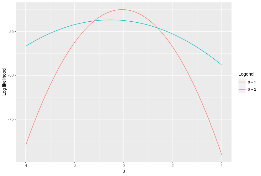
I tend to find that I have a better grasp of the maths if I have some feeling for the numbers at hand. As an example, I’ve generated samples of 10 observation from different normal distributions. As a comparison, I’ve used two normal distributions centred on 0 with standard deviations of 1 and 2 respectively:
set.seed(3.14) #ensure that results are reproducible
small_var <- rnorm(10) #generate 10 IID observations from the standard normal distribution
large_var <- rnorm(10, sd = 2) #double the standard deviation
In this example, the inferred parameter $\theta$ is the mean $\mu$. Log likelihood is calculated here using different values of $\mu$. The peak log likelihood occurs at the maximum likelihood estimator (MLE) of $\mu$. Note that log likelihood curve is sharper when $\sigma$ is smaller.
The score is the gradient of this curve. Though it can be calculated analytically in this case, I’ve approximated the derivative numerically using a simple central difference:
score <- function(mu, st_dev, sample){
  lhood_minus <- log_likelihood(mu-0.01, st_dev, sample)
  lhood_plus <- log_likelihood(mu+0.01, st_dev, sample)
  return((lhood_plus-lhood_minus)/0.02)
}
Which looks like this:
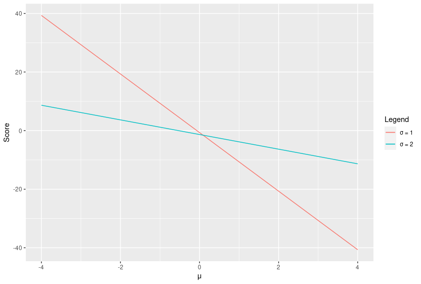
In the case of the normal distribution, the score forms a nice straight line. Notice that this line is steeper for $\sigma = 1$. However, we’re really only interested in what happens at the true value of $\theta$. In other words, the value of the score at $\mu = 0$.
Fisher Information
Imagine generating many of these random samples and calculating the value of this intercept (at the true value of $\theta$) each time. The asymptotic variance of all the observations is the Fisher Information. More formally:
$$ I_{X}\left( \theta \right) =Var_{\theta}\left( s\left( X,\theta \right) \right) $$
Since the expected value of the score is zero:
\[\begin{align*} Var_{\theta }\left( s\left( X,\theta \right) \right) &= E_{\theta}\left( s-E_{\theta}\left( s\right) \right) ^{2}\\ &= E_{\theta}\left( s^{2}\right) \end{align*}\]Note that the Fisher information above is for the entire sample X. However, it can also be calculated for an individual observation such as $X_{1}$. A very useful property of Fisher information is that these values are closely related. For independent, identically distributed (IID) samples:
$$ I_{X}(\theta) = nI_{X_{i}}(\theta) $$
where $n$ is the sample size.
Calculating Fisher Information
The normal distribution has two parameters and so its Fisher information actually takes the form of a diagonal 2*2 matrix. I’ll derive the Fisher information with respect to $\mu$. The easiest way to approach this calculation is to calculate it for a single observation, using the sample size property given above:
\[\begin{align} L\left( x,\theta \right) &=\dfrac{1}{\sigma \sqrt{2\pi }}e^{-\dfrac{1}{2}\left( \dfrac{x-\mu }{\sigma }\right) ^{2}} \\ \\ \ln L\left( x,\theta \right) &=-\ln \left( \sigma \sqrt{2\pi }\right) -\dfrac{1}{2\sigma ^{2}}\left( x-\theta \right) ^{2} \\ \\ s\left( x,\theta \right) &=\dfrac{\partial }{\partial \theta }\left( -\log \left( \sigma \sqrt{2\pi }\right) -\dfrac{1}{2\sigma ^{2}}\left( x-\theta \right) ^{2}\right) \\ &=\dfrac{\partial }{\partial \theta }\left( -\dfrac{1}{2\sigma ^{2}}\left( x^{2}-2\theta x+\theta ^{2}\right) \right) \\ &=\dfrac{1}{2\sigma ^{2}}\left( -2\theta +2x\right) \\[3px] &= \dfrac{\theta -x}{\sigma ^{2}} \\ \\ I_{X_{i}}\left( \theta \right) &=E_{\theta }\left[ \left( s\left( x,\theta \right) \right) ^{2}\right] \\ &=E_{\theta }\left[ \dfrac{\left( \theta -x\right) ^{2}}{\sigma ^{4}}\right] \\ &=E_{\theta }\left[ \dfrac{\sigma ^{2}}{\sigma ^{4}}\right] \\ &=\dfrac{1}{\sigma ^{2}}\end{align}\]There’s actually an easier way to calculate the Fisher information here using the second derivative, but I’ll save that for the next post.
As you can see, a smaller variance results in more accurate estimates of $\mu$ and therefore a lower Fisher Information (all things being equal). This is for the case of a single observation. Considering there are 10 observations here, the sample Fisher information is $n*\dfrac{1}{\sigma ^ {2}} = \dfrac{10}{\sigma ^ {2}}$. This corresponds to 10 and 2.5 for $\sigma$ = 1 and 2 respectively.
As a final step, I decided to demonstrate the maths in action by estimating the Fisher information over many samples. R makes this too easy!
for (i in c(1:100000)){
  small_var <- rnorm(10) #generate 10 IID observations from the standard normal distribution
  large_var <- rnorm(10, sd = 2) #double the standard deviation

  info_small[i] <- scores_squared(0, 1, small_var)
  info_large[i] <- scores_squared(0, 2, large_var)

  ave_small[i] <- mean(info_small[1:i])
  ave_large[i] <- mean(info_large[1:i])
}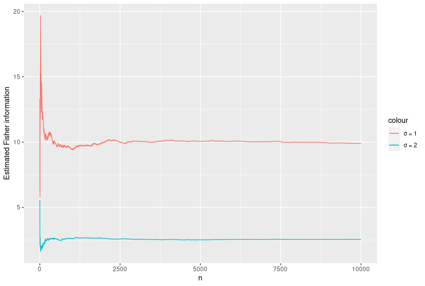
The estimated Fisher Information seems to converge to the calculated value. Isn’t it good when maths does what it’s supposed to!